import numpy as np
x = np.array([1, 2, 3])
sum_of_products = (x**2).sum()
print(sum_of_products)14Ever needed to compare lots of variables and missing data made things super slow?
A surprisingly wide range of measures that are core to data science can be accelerated with the use of matrix multiplication. You just need to get creative when reformulating your computation.
But real-world data has missing values and these can make matrix multiplication useless. Does that mean one must resort to inefficient for-loops to keep track of missing values?
No. Using Numpy masked arrays one can still reap the benefits of matrix multiplication whilst making full use of one’s data.
Here I demonstrate the use of numpy masked arrays for the efficient calculation of percentage agreement among many binary variables.
In this post I cover:
The covariance matrix is another measure we can efficiently compute using MM and masked arrays. I am leaving that for another post where I also describe existing solutions (coming soon).
The solution I describe here for efficient computation of percentage agreement is not something in any major Python package.
I also refer to a similar implementation of Cohen’s kappa I coded (in #sec-masked-arrays). Cohen’s kappa with efficient matrix-based handling of missing values is also missing in major Python packages.
But before we get to all that, let’s talk about matrix multiplication (MM).
As implemented in most popular packages like Python’s Numpy, MM let’s you rapidly calculate sums-of-products for many pairs of variables. So let’s start with sums-of-products.
Here is a single variable and it’s sum-of-products:
import numpy as np
x = np.array([1, 2, 3])
sum_of_products = (x**2).sum()
print(sum_of_products)14Now we consider another variable y and calculate the sum-of-products between x and y:
y = np.array([3, 2, 1])
products = np.multiply(x, y)
sum_of_products = products.sum()
print(products)
print(sum_of_products)
[3 4 3]
10Now we package our x and y as the column vectors of a single matrix:
X = np.array([[1, 3],
              [2, 2],
              [3, 1]])
number_observations, number_variables = X.shape
print(f"{number_observations} observations (rows)")
print(f"{number_variables} variables (columns)")
3 observations (rows)
2 variables (columns)Why did with do this? If you matrix multiply X with itself you get something interesting:
S = np.dot(X.transpose(), X)
print(S)
[[14 10]
[10 14]]S[0,0] is the sum-of-products of x with itself. S[0,1] is the sum-of-products of x with y. S[1,0] is also the sum-of-products of x with y. And S[1,1] is the sum-of-products of y with itself.
In other words, matrix multiplication (MM) gives you the sum-of-products for every pairwise comparison.
And as mentioned earlier, MM is computed very quickly using packages like Numpy.
But why do we care about sums-of-products for every pairwise comparison?
So many interesting measures/statistics can be reformulated as an efficient sequence of MM.
So with just a little bit of cleverness you can turn your very inefficient for-loops into a very efficient sequence of matrix operations.
Imagine that 8 people filled out a survey consisting of 4 yes/no items:
import pandas as pd
X = np.array([[0, 0, 0, 0, 1, 1, 1, 1],
              [0, 0, 0, 0, 1, 1, 1, 1],
              [0, 1, 0, 1, 0, 1, 0, 1],
              [1, 1, 1, 1, 0, 0, 0, 0]]).transpose()

col_labels = ['Item ' + str(i) for i in range(1,5)]
row_labels = ['Person ' + str(i) for i in range(1,9)]
print(pd.DataFrame(X, columns=col_labels, index=row_labels))
Item 1 Item 2 Item 3 Item 4
Person 1 0 0 0 1
Person 2 0 0 1 1
Person 3 0 0 0 1
Person 4 0 0 1 1
Person 5 1 1 0 0
Person 6 1 1 1 0
Person 7 1 1 0 0
Person 8 1 1 1 0You want to know if there are associations among these items.
A glance at this stylized data set suffices.
Item 1 is perfectly positively associated with item 2 in this sample; 100 percent of the responses are in agreement.
Item 1 is has no association with item 3 in this sample; guessing someone’s response to item 3 based their response to 1 is no better than a coin flip (50 percent).
Item 1 is perfectly negatively associated with item 4; 0 percent of the responses are in agreement.
If you have a much larger data set, you might decide to use for-loops like this:
def pa_loop(X):
    number_samples, number_variables = X.shape
    percent_agreement = np.zeros((number_variables, number_variables))
    for item_a in range(number_variables):
        for item_b in range(item_a+1, number_variables):
            percent_agreement[item_a, item_b] = (X[:, item_a]==X[:, item_b]).sum()
    percent_agreement /= number_samples
    return(percent_agreement)
But this can be slow for large data sets:
from time import perf_counter
number_samples, number_variables = 1000, 1000
X = np.random.choice([0., 1.], size=(number_samples, number_variables), replace=True)
tic = perf_counter()
percent_agreement = pa_loop(X)
toc = perf_counter()
print(f"Computing all pairwise percentage agreements took {toc-tic:0.4f} seconds.")
Computing all pairwise percentage agreements took 1.8570 seconds.This may not seem so bad. But consider that
How can we use matrix multiplication to speed things up? We’ll have to use some tricks but it’s not that hard.
Here is a simple case with yes and no responses for 2 items coded as 1s and 0s respectively:
| item 1 | item 2 | agreement | yes-yes | no-no |
|---|---|---|---|---|
| 0 | 0 | 1 | 0 | 1 |
| 0 | 1 | 0 | 0 | 0 |
| 1 | 0 | 0 | 0 | 0 |
| 1 | 1 | 1 | 1 | 0 |
What we want is a column like agreement above whose sum (2) gives us the number of agreements. We then divide 2 by 4 to get 50-percent agreement.
Treating item 1 as a row vector and item 2 as a column vector, we can perform matrix multiplication to get the sum of yes-yes (1). As an intermediate step in matrix multiplication, our 2 vectors are multiplied value-by-value giving us the yes-yes column above. Summing is the final step of matrix multiplication (1).
Agreements can be either yes-yes or no-no so we still need to obtain that sum before we can measure number of agreements. That’s easy. We simply flip the values in item 1 and item 2 from 0 to 1, and 1 to 0:
\[ new = \lvert old-1 \rvert \]
Matrix multiplication of these complementary vectors for item 1 and item 2 (not shown here) gives us our sum of no-no, whose intermediate step is the no-no column above.
The above example is for 2 items but the power of matrix multiplication is that we are multiplying matrices – as many items as we want. And the result is a matrix of all pairwise comparisons. In other words, we can obtain a matrix of percentage agreement for all pairwise comparisons using a simple sequence of matrix-based operations, like this:
def pa_vect(X):
    number_samples, number_variables = X.shape # (n x k)
    yesYes = np.dot(X.transpose(), X)          # counts of yes-yes (k x k)
    np.abs(X-1, out=X)                         # [0,1] -> [1,0]
    noNo = np.dot(X.transpose(), X)            # counts of no-no   (k x k)
    S = yesYes + noNo                          # counts of agreements (k x k)
    A = S / number_samples                     # percentage agreements (k x k)
    return(A)
How much faster is this compared to the loop-based computation?
number_samples = 1000
number_variables = [10, 50, 100, 500, 1000]
seconds = np.zeros((len(number_variables), 2))
iterations = 36

for i, nvl in enumerate(number_variables):
    for _ in range(iterations):
        X = np.random.choice([0., 1.], size=(number_samples, nvl), replace=True)
        tic = perf_counter(); percent_agreement = pa_loop(X); toc = perf_counter()
        seconds_loop = toc-tic
        tic = perf_counter(); percent_agreement = pa_vect(X); toc = perf_counter()
        seconds_vect = toc-tic
        seconds[i, 0] += seconds_loop
        seconds[i, 1] += seconds_vect

seconds /= iterations

df = pd.DataFrame(seconds,
                  columns=['loop','matrix-based'],
                  index=number_variables)
df| loop | matrix-based | |
|---|---|---|
| 10 | 0.000217 | 0.000156 |
| 50 | 0.005415 | 0.000235 |
| 100 | 0.021027 | 0.000606 |
| 500 | 0.500720 | 0.006657 |
| 1000 | 1.909704 | 0.022183 |
Let’s examine the speed up graphically:
import matplotlib.pyplot as plt

df.plot(loglog=True, xlabel="Number of variables", ylabel="Seconds")
plt.show()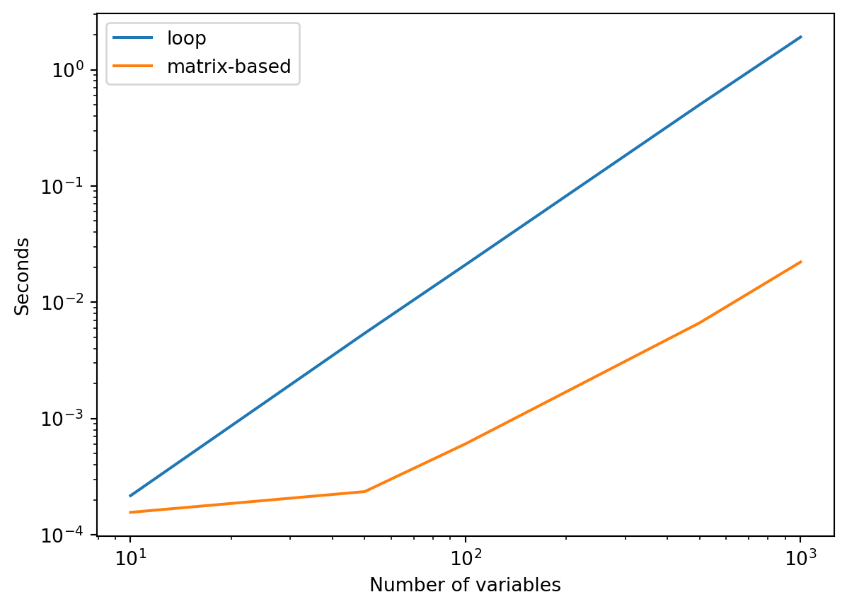
Matrix-based computation is definitely faster!
How much faster exactly?
Dividing the time taken by loop-based computation by the time taken by matrix-based computation gives us a speed-up. The larger the number the stronger the advantage for matrix-based computation:
speed_up = seconds[:,0] / seconds[:,1]
plt.semilogx(number_variables, speed_up)
plt.xlabel("Number of variables")
plt.ylabel("Speed advantage")
plt.title("Matrix-based operation beats loops by miles")
plt.show()
Numpy is efficient because its data structures (matrices, vectors) have homogeneous elements. Everything in a numpy matrix for example is int32 or whatever data type you set it to be (e.g., float64).
If you have an element that is undefined for some reason, like a missing value for example, then it is usually represented as nan. That stands for not-a-number and is common in programming languages. Note that nan is only defined for floating point data types.
For convenience, let’s assign a variable to represent np.nan so we do not have to type np.nan all the time:
M = np.nanNow let’s see why missing values in Numpy (nan) can be a problem for our MM solutions.
If we do any arithmetic that involves a nan we get a nan as a result:
print(f"10 + nan is {10 + M}")
print(f"23 * nan is {23 * M}")
10 + nan is nan
23 * nan is nanSo if we do matrix multiplication, we will get nan for every pair that has at least one nan:
x = np.array([1, 2, 3, 4]).reshape((4,1))
y = np.array([1, 2, 3, M]).reshape((4,1))
mm = np.dot(x.transpose(), y)
print(f"matrix multiplication of {x.flatten()} and {y.flatten()} is {mm}.")
matrix multiplication of [1 2 3 4] and [ 1. 2. 3. nan] is [[nan]].Now let’s see how we can deal with missing values in data sets.
There are simple cases which are uncommon, and there are complex cases which are common.
Here is an extremely simple case:
X = np.array([[0, 0, 0, 1],
              [0, 0, 1, 1],
              [1, 1, 0, 0],
              [1, 1, 1, 0],
              [M, M, M, M]])
col_labels = ['Item ' + str(i) for i in range(1,5)]
row_labels = ['Person ' + str(i) for i in range(1,6)]
print(pd.DataFrame(X, columns=col_labels, index=row_labels))
Item 1 Item 2 Item 3 Item 4
Person 1 0.0 0.0 0.0 1.0
Person 2 0.0 0.0 1.0 1.0
Person 3 1.0 1.0 0.0 0.0
Person 4 1.0 1.0 1.0 0.0
Person 5 NaN NaN NaN NaNHere we can perform listwise deletion, with no loss of information:
X[:-1,:]array([[0., 0., 0., 1.],
[0., 0., 1., 1.],
[1., 1., 0., 0.],
[1., 1., 1., 0.]])But the missing values in real data will often be in different records for different variables. Here is an extreme case:
X = np.array([[0, 0, M, M],
              [0, 0, M, M],
              [1, 1, M, M],
              [1, 1, M, M],
              [0, M, 0, M],
              [0, M, 1, M],
              [1, M, 0, M],
              [1, M, 1, M],
              [0, M, M, 1],
              [0, M, M, 1],
              [1, M, M, 0],
              [1, M, M, 0]])
If we do listwise deletion we end up with no data.
What we want is pairwise deletion instead of listwise deletion. We want to only exclude samples on a pairwise basis in order to retain the most information.
This is pretty straightforward with our loop-based code. We simply add list comprehensions inside the inner loop, which excludes samples whenever a value is missing for one of the pairs under consideration:
import math

def pa_loop_missing(X):
    _, number_variables = X.shape
    percent_agreement = np.zeros((number_variables, number_variables))
    for item_a in range(number_variables):
        for item_b in range(item_a+1, number_variables):
                x = X[:, item_a]
                y = X[:, item_b]
                # remove observations where missing for either x or y
                products = [a*b for a, b in zip(x,y)]
                nx = [xi for xi, pi in zip(x, products) if not math.isnan(pi)]
                ny = [yi for yi, pi in zip(y, products) if not math.isnan(pi)]
                sumA = sum([va==vb for va, vb in zip(nx, ny)])
                totA = len(nx)
                percent_agreement[item_a, item_b] = [sumA / totA if totA > 0 else math.nan][0]
    return(percent_agreement)

pa_loop_missing(X)
array([[0. , 1. , 0.5, 0. ],
[0. , 0. , nan, nan],
[0. , 0. , 0. , nan],
[0. , 0. , 0. , 0. ]])This works but as we will see in Section 5, this solution is very slow. That is not a surprise since we now effectively have 3 nested loops.
And if we try out matrix-based solution we end up no result except for the agreement of the first item with itself:
pa_vect(X)array([[ 1., nan, nan, nan],
[nan, nan, nan, nan],
[nan, nan, nan, nan],
[nan, nan, nan, nan]])Of course. We already knew this.
In fact, it seems impossible to avoid for-loops if one wants to perform pairwise deletion.
Or is it?
As it turns out, numpy masked arrays effectively performs pairwise deletion when a matrix multiplication is performed!
Despite being very valuable, this feature of masked arrays is not something that appears to be commonly appreciated in discussions of what makes masked arrays useful.
For example, see the top-rated responses to this Stack Overflow query on Why are Numpy masked arrays useful? Practical examples like what’s presented here are hard to find.
So let’s make sure pairwise deletion is indeed performed using a matrix multiplication of masked arrays. I was not sure myself and had to check using numerous examples. Here is a really simple example I showed you before:
X = np.array([[0, 0, M, M],
              [0, 0, M, M],
              [1, 1, M, M],
              [1, 1, M, M],
              [0, M, 0, M],
              [0, M, 1, M],
              [1, M, 0, M],
              [1, M, 1, M],
              [0, M, M, 1],
              [0, M, M, 1],
              [1, M, M, 0],
              [1, M, M, 0]])

col_labels = ['Item ' + str(i) for i in range(1,X.shape[1]+1)]
row_labels = ['Person ' + str(i) for i in range(1,X.shape[0]+1)]

print(pd.DataFrame(X, columns=col_labels, index=row_labels))
Item 1 Item 2 Item 3 Item 4
Person 1 0.0 0.0 NaN NaN
Person 2 0.0 0.0 NaN NaN
Person 3 1.0 1.0 NaN NaN
Person 4 1.0 1.0 NaN NaN
Person 5 0.0 NaN 0.0 NaN
Person 6 0.0 NaN 1.0 NaN
Person 7 1.0 NaN 0.0 NaN
Person 8 1.0 NaN 1.0 NaN
Person 9 0.0 NaN NaN 1.0
Person 10 0.0 NaN NaN 1.0
Person 11 1.0 NaN NaN 0.0
Person 12 1.0 NaN NaN 0.0Clearly the sum of products between item 1 and itself should be 6, between item 1 and 2 should be 2, between item 1 and 3 should be 1, and between item 1 and 4 should be 0. You easily calculate the rest yourself.
Let’s see if matrix multiplication with masked arrays is consistent with pairwise deletion.
The first step is to import the masked array module, and convert X to a masked array such that nan values are identified as masked:
import numpy.ma as ma

R = ma.masked_invalid(X)
Now the rest is the easy. The masked array module contains almost all of the same functionality as numpy itself. So for example we can write ma.dot() instead of np.dot():
yesYes = ma.dot(R.transpose(), R)

print(pd.DataFrame(yesYes, columns=col_labels, index=col_labels))
Item 1 Item 2 Item 3 Item 4
Item 1 6.0 2.0 1.0 0.0
Item 2 2.0 2.0 NaN NaN
Item 3 1.0 NaN 2.0 NaN
Item 4 0.0 NaN NaN 2.0Fantastic! Pairwise deletion without for loops!
But is this fast? Can we still get those juicy speed gains using matrix multiplication on masked arrays?
Let’s find out. First let’s re-code our function for matrix-computation of percentage agreement to perform all operations on a masked-array version of the data:
def pa_vect_missing(X):
    R = ma.masked_invalid(X)                # (n x k)
    yesYes = ma.dot(R.transpose(), R)       # counts of yes-yes (k x k)
    F = ma.abs(R-1)                         # [0,1] -> [1,0]
    noNo = ma.dot(F.transpose(), F)         # counts of no-no   (k x k)
    S = yesYes + noNo                       # counts of agreements (k x k)
    valid = np.ones_like(R)                 # valid responses (n x k)
    valid[ma.getmaskarray(R)] = 0
    N = np.dot(valid.transpose(), valid)    # valid count (k x k)
    A = ma.multiply(S, N**-1)               # percentage agreement (k x k)
    return(A)
And now let’s compare our new loop- and matrix-based functions across a range of data sizes. Here I simulate binary responses with 20-percent missing data on average, randomly dispersed across sample and variable:
rng = np.random.default_rng(seed=12345)

responses, probs = [0., 1., M], [.4, .4, .2]
number_samples_large = 1000
number_variables_large = [10, 50, 100, 500, 1000]
seconds_missing = np.zeros((len(number_variables_large), 2))
iterations = 2

for i, nvl in enumerate(number_variables_large):
  for _ in range(iterations):
    X = rng.choice(responses,
                   size=(number_samples_large, nvl),
                   replace=True,
                   p=probs)
    tic = perf_counter()
    percent_agreement = pa_loop_missing(X)
    toc = perf_counter()
    seconds_loop = toc-tic
    tic = perf_counter()
    percent_agreement = pa_vect_missing(X)
    toc = perf_counter()
    seconds_vect = toc-tic
    seconds_missing[i, 0] += seconds_loop
    seconds_missing[i, 1] += seconds_vect

seconds_missing /= iterations

df_missing = pd.DataFrame(seconds_missing,
                          columns=['loop','vectorized'],
                          index=number_variables_large)

df_missing.plot(loglog=True, xlabel="Number of variables", ylabel="Seconds")
plt.show()

df_missing.to_csv("tests_missing.csv")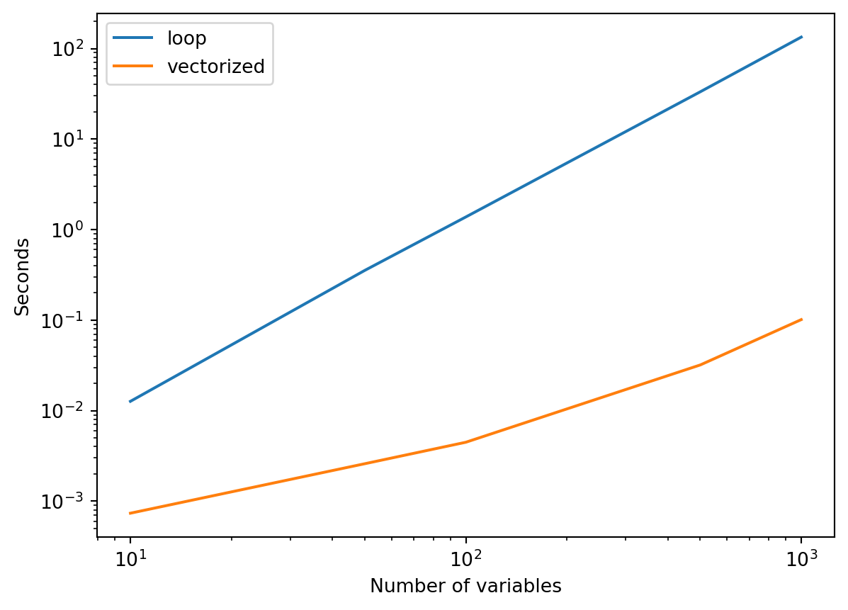
Wow, is that an almost 1000-fold speed advantage for matrix-based computation?
Again let’s show ratios of time taken to see:
speedup = seconds_missing[:,0]/seconds_missing[:,1]

# Max speed-up rounded, for title
power = np.floor(np.log10(speedup.max()))
lower = np.floor(speedup.max() / 10**power) * 10**power

import matplotlib.ticker as mticker

fig, ax = plt.subplots(figsize=(7, 2.7), layout="constrained")
ax.plot(number_variables_large,
        speedup,
        color='blue',
        linewidth=3,
        linestyle='-',
        marker='o')
ax.set_xscale("log")
ax.set_xlabel("Number of variables")
ax.set_ylabel("Speed advantage")
ax.set_title("Vectorization up to ")
ax.set_title(f"Vectorized code more than {lower:.0f}" + r"$\bf{X}$ faster than loops")
ylim = ax.get_ylim()
ax.set_ylim((1,ylim[1]))
ticks_loc = ax.get_yticks().tolist()
ax.yaxis.set_major_locator(mticker.FixedLocator(ticks_loc))
ytickLabels = [str(int(n)) + r"$\bf{X}$" for n in ticks_loc]
ax.set_yticklabels(ytickLabels)
plt.show()

fig.savefig("tests-missing.svg")
Yes, indeed. An almost 1000-fold speed advantage!
Obviously you’d want to run a speed test multiple times but I do not think minor changes in computer state or exact data would change all that much. Nonetheless, you may want to know about my set up. I ran this on an AMD Ryzen 7 5800H with 32GB ram.
Oh yeah, I also mentioned something about Cohen’s kappa coefficient. This is something you may want to consider using if you want to take into the degree to which agreements can happen by chance. Cohen’s kappa is currently implemented in scikit-learn but only handles single pairs. If you wanted to measure kappa among a large number of variables using scikit-learn then you’d have to put their function into a nested loop.
So I wrote a matrix-based version of cohen’s kappa that can handle missing values efficiently and I put it in this GitHub repo. It is basically like pa_vect_missing() but with some additional lines of code. So if you understood the discussion so far, then understanding my function for Cohen’s kappa should be straightforward.
I do not think that my solution for Cohen’s kappa would be useful for scikit-learn, as Cohen’s kappa is primarily used there for model comparison with ground-truth labels. Unless you wanted to obtain a detailed picture of categorization errors among hundreds of thousands of models … I used my code for simple data exploration.
If you want to implement your own solution, you may want to know about Numpy optimization. Especially if you’re not getting the gains you hoped for.
I highly recommend the blog post by Shih-Chin on this topic. It is well written and informative!
Here I point out one little detail you might have missed in the my data-generation code:
Xa = np.random.choice([0., 1.], size=(1000, 1000), replace=True)
Xb = np.random.choice([0,  1],  size=(1000, 1000), replace=True)
print(f"Xa has data type {Xa.dtype}.")
print(f"Xb has data type {Xb.dtype}.")
Xa has data type float64.
Xb has data type int64.You might remember that the presence of missing values will automatically cast data type to float. So all the data in Section 4 were float64.
When I wrote about computation without missing values (Section 3), I was careful to keep this consistent and also use floating value: like Xa in the above code and not like Xb! Why be so careful?
As it turns out, this can have an effect on computational speed.
Let’s see how long it takes to do matrix multiplication on float64 with 2 different orders of operation:
import timeit
iterations = 1000

setup = """
import numpy as np
Xa = np.random.choice([0., 1.], size=(1000, 1000), replace=True)
"""
tf = timeit.Timer("np.dot(Xa.transpose(), Xa)", setup=setup)
sec_order_1 = tf.timeit(number=iterations)/iterations
tf = timeit.Timer("np.dot(Xa, Xa.transpose())", setup=setup)
sec_order_2 = tf.timeit(number=iterations)/iterations
print(f"np.dot(Xa.transpose(), Xa) took {sec_order_1} seconds.")
print(f"np.dot(Xa, Xa.transpose()) took {sec_order_2} seconds.")
np.dot(Xa.transpose(), Xa) took 0.00926350842500142 seconds.
np.dot(Xa, Xa.transpose()) took 0.008056458486000338 seconds.A reader that is familiar with matrix computation will notice that np.dot(Xa, Xa.transpose()) does not make sense for our data. The X used in this blog post has samples along rows and variables along columns. So np.dot(Xa, Xa.transpose()) would give comparisons of samples not variables. If we had constructed X so that rows and columns were opposite then np.dot(Xa, Xa.transpose()) would give us the desired comparisons of variables.
I included both orders because based on Shih-Chin discussion of Numpy, I suspected there might be a difference. There is a small difference so I decided to stick to X with variables along columns (and use np.dot(Xa.transpose(), Xa)). That format is in keeping with Pandas format and most data science.
Now what happens when our data X is int64 instead of float64?
iterations = 50
setup = """
import numpy as np
Xb = np.random.choice([0,  1],  size=(1000, 1000), replace=True)
"""
tf = timeit.Timer("np.dot(Xb.transpose(), Xb)", setup=setup)
sec_order_1 = tf.timeit(number=iterations)/iterations
tf = timeit.Timer("np.dot(Xb, Xb.transpose())", setup=setup)
sec_order_2 = tf.timeit(number=iterations)/iterations
print(f"np.dot(Xb.transpose(), Xb) took {sec_order_1} seconds.")
print(f"np.dot(Xb, Xb.transpose()) took {sec_order_2} seconds.")
np.dot(Xb.transpose(), Xb) took 1.0244241412799966 seconds.
np.dot(Xb, Xb.transpose()) took 0.4779843139599689 seconds.The most striking thing is that, regardless or operation order, computation of int64 data is much slower!
Even if your data are naturally integers it might make sense to cast them as float! That of course does not apply with missing data (contains nan), but your data might be originally integer in another scenario.
The second striking thing is that np.dot(Xb, Xb.transpose()) is markedly faster than np.dot(Xb.transpose(), Xb)!
If your data are integer and you do not have missing values then you will want to construct your data with variables along rows and perform matrix multiplication with the transposed data on the right-hand side!
I should mention one more issue that is not computational but statistical. This discussion ignores how statistical inference works when we are performing pairwise deletion. If you are simply exploring your data or trying out different machine learning methods, then that’s not such an issue. But keep in mind that the effect of pairwise deletion on inference is likely to be tricky.
If you need to compute a measure/statistic for all pairwise comparisons among a large set of variables, then you can probably speed things up a lot with matrix multiplications. It may take some creativity, but hopefully this blog post can provide some inspiration.
If you have missing data then matrix multiplication using Numpy masked arrays does pairwise deletion efficiently and that’s very useful to know!
If you do decide to try out a similar solution for your measure/statistic, pay heed to Section 6. And watch out for the Numpy acceleration package Jax. While it currently does not support masked arrays, perhaps it or some external package using Jax will do so in the future. That could potentially make the gains described here even greater.
The solution I present here for percentage agreement and Cohen’s kappa is not currently implemented in any major Python package.
Finally, watch out for my next post on how missing data are dealt with by current solutions that measure the covariance matrix, and why that matters.